Dijkstra’s Algorithm
A Gentle introduction to Dijkstra’s algorithm
AIM: To understand Dijkstra’s algorithm really well and implement it in Java.
Route: We will use plain english, a bit of pseudocode and python to introduce the algorithm and finally implement it using Java.
If you are visiting related Graph topic after a while, you may read this quick introduction to Graph concepts by Hacker Earth.
Dijkstra’s algorithm, lets you answer “What’s the shortest path to X?” for weighted graphs. Remember, BFS Algorithm does the same thing for unweighted graphs.
Dijkstra’s algorithm only works with directed graphs which does not have any negative cycles. The the algorithm works for graphs with positive cycles. See this stackoverflow link for a nice discussion on the topic.
Dijkstra’s algorithm doesn’t work for graphs with negative weight edges. For graphs with negative weight edges, Bellman–Ford algorithm can be used.
Working with Dijkstra’s Algorithm
When you work with Dijkstra’s algorithm, each edge in the graph has a number associated with it. These are called weights.
Given below is a weighted graph where numbers on the edges denotes the travel time to reach from one vertex to another. If we apply the normal BFS algorithm on this graph, the shortest path from Start to Finish would be (Start)->(A)->(Finish) or even (Start)->(B)->(Finish). The travel time for this path is 6 + 1 = 7 minutes (or 2 + 5 = 7 mins). On an detailed eyeball inspection we can see that there is a path with shorter travel time, (Start)->(B)->(A)->(Finish) which has a total travel time of 2 + 3 + 1 = 6 minutes.
         ( A )
       `#``#` \
      6/   |   \1
      /    |    \
     /    3|     \
    /      |     `#`
(Start)    |   (Finish)
   \       |      `#`
    \      |      /
    2\     |     /5
      \    |    /
       \   |   /
       `#` |  /
         ( B )

 `#` indicates an Arrow.
Dijkstra Algorithm consists of a Setup phase and a Probing phase.
Setup Phase : During the setup phase you initialize a costs_table. It is a dictionary or hashtable containing entries for all the nodes except the Start node, the key will be the Node and the value will be the cost to reach each node, following the shortest path. Initially, the costs_table will be initialized using following rule, only Nodes that has a direct path from Source node will have an entry with respective cost. All other Nodes will have an entry with cost set to infinity. That’s because, at this point, we don’t know the Shortest path to those Nodes. If this sounds confusing to you, don’t worry, I am sure you will get it in the next section were we work through the example Graph. Just remember that in the Setup phase, we construct the costs_table.
Probing Phase : Durign the probing phase we traverse through each Node of the Graph in search of more optimal paths to it’s neighbouring nodes. As and when we find an optimal path to a Node, the costs_table is updated with that information. There is also a parents_table to keep track of the Shortest path to a given node. We will talk more about that later. The Probing phase comes to an end when we do not have any Node left for visiting.
During the probing phase a two step process is followed.
Step 1: Identify the cheapest Node.
Step 2: Perform relaxation on each of the neighbouring nodes of the cheapest Node. During the relaxation process, we check whether the path to a neighbouring node is cheaper if we go through the current cheapest node . If yes, the costs_table entry is updated with the new cost. The parents_table is also updated to indicate that the current cheapest node is the parent of the neighbouring node under scanner.
When you are done with the probing phase, the cost of shortest path from the starting node to all other nodes will be available in costs_table. Similarly, the actual shortest path from Start to Finish (or any Node) can be deduced by backtracking on the parents_table. You will understand it better when you see the code where we print the shortest path.
Applying Dijkstra’s Algorithm on the example Graph
Let’s apply Dijkstra’s algorithm on our example Graph and see whether we are able to get the same shortest path that we got through manual inspection.
Setup Phase :
In the setup phase we have to initialize the costs_table. The rule to be followed is that, make an entry for every node except the starting node in the costs_table. For the nodes that are having direct edge from the Start node, make an entry with the edge weight as the cost, because that’s the cost required to reach that node. For all other nodes, set the cost as “infinity”, because we don’t know whats the cost to reach them. Following this rule, we initialise the costs_table as below.
costs_table = {}
costs_table["A"] = 6
costs_table["B"] = 2
costs_table["Finish"] = infinity
Ideally, code should be written to do this initialization in a generic way. But, to keep thinks simple, we are initializing costs_table this way, which is very specific for the Graph that we have taken as example. In subsequent iterations, we will try to generalize this code as well.
Probing Phase :
Step 1: Pick the cheapest node from costs_table. The generic algorithm to find the cheapest node is very simple. We just iterate over the entire costs_table and pick the least cost node that is not yet processed/visited.
At the very beginning of the iteration, the entries in costs_table are simple entries, meaning they are the weights of edges that connect the Start node to the respective nodes.
      Node   | Total cost to reach the Node
      A      | 6
      B      | 2
      Finish | Infinity (infinity because there is no direct path from Start to Finish and we do not know the actual distance)
From the costs_table we pick least cost node, which is Node B.
Step 2: Perform relaxation or Update the costs_table for each of the neighbours of the least_cost_node (currently Node B). Formula used will be new_cost = cost_to_reach_least_cost_node + neighbours_edge_weight. We replace the costs_table entry only if new_cost is less than the existing cost. In otherwords, we replace the costs_table entry only if new path is better than the existing path.
Since B is the least_cost_node, we get all neighbours of B, using graph[B].keys(). This will return Node A and Node Finish. So, we will perform relaxation on Node A and Node Finish. Current costs_table entry for Node A is 6, and the new_cost is costs_table[B] + edge_weight (of path from B to A) = 2 + 3 = 5. Since, new_cost is less that current entry we update the costs_table for Node A with the new value.
      Node   | Total cost to reach the Node
     `A      | 5`
      B      | 2
      Finish | Infinity (infinity because there is no direct path and we do not know the actual distance)
For the Node Finish, the current cost is Infinity. new_cost = costs_table[B] + edge_weight (of path from B to Finish) = 2 + 5 = 7.
      Node   | Total cost to reach the Node
      A      | 5
      B      | 2
     `Finish | 7`
One thing to keep in mind is that the costs_table entry is an aggregation of edge weights based on the shortest known path to a Node. As and when we discovery a new optimal path, the costs_table entry is updated to reflect the latest aggregate cost.
Step 3: Add B to processed nodes list. Update parents_table entry for Node A and Node Finish to point to Node B, which is the parent node for A and Finish. So we set, parents_table[A]=’B’ and parents_table[Finish]=’B’.
Step 4: Pick the next least cost node from costs_table. This time, it will return A. Node B is not returned because, B is in the processed_nodes list.
Step 5: From here we can loop back to Step 2. But for the purpose of illustration, we will walk through the entire execution flow. So, in this step we update the costs_table for each of the neighbours of Node A based on the formula explained in Step 2. Node A has only one neighbour, Node Finish. The current costs_table entry for Node Finish is 7. The new_cost = costs_table[A] (or cost to reach A) + edge_weight (from A to Finish) = 5 + 1 = 6. Hurrah!, we found a new path which is better than the currenty known best path. It takes only 6 mins to reach Finish through A compared to the previous time which was 7 mins. So we update the costs_table accordingly.
      Node   | Total cost to reach the Node
      A      | 5
      B      | 2
     `Finish | 6`
Step 6: We add A to processed_nodes list. Update parents_table entry for Finish. Basically, we will set parents_table[Finish]=’A’ to indicate that the path to Finish is through A.
Step 7: We again call find_lowest_cost_node, which will return the Finish node.
Step 8: There are no neighbours for Finish node. So, Perform relaxation phase gets skipped.
Step 9: We again go back to find_lowest_cost_node. This time it will return None, as all of the nodes are in the processed_nodes list. That marks the end of Dijkstra’s algorithm execution. At this point, costs_table will have the cost of shortest path from Start node to any given node. For example, costs_table[Finish] will give cost of Shortest path from Start node to Finish node.
Step 10: In order to print the actual shortest path, we need to backtrack using the parents_table. parents_table[‘Finish’] will give parent of Finish. We will have to do this for every parent node, until we reach the Start node. This can be seen in action under the Print the results section of python code.
Datastructures required to implement Dijkstra’s Algorithm
- A HashTable which we call
Graphto represent the Graph. It is actually a HashTable of HashTable because we have to store the weights of the edges as well. I will explain it in detail later. - A HashTable which we call
costs_tableto represent the cost to reach a node. If the cost for a Node is unknown we put infinity. - A HashTable which we call the
parents_tableto track the parent node of a given node. - A List which we call the
processed_nodesto keep track of the visited or processed nodes.
How do we represent the Graph with weights using HashTable? Based on our earlier strategy, we would have represented the connection from “Start” to A and B as follows,
graph = {}
graph["Start"] = ["A", "B"]
You may have a look at the visualization here.
But, where do we put the weight corresponding to the edges Start->A and Start->B? Again, hashtable comes to our rescue. Instead of placing an Array within a HashTable entry, we are going to place a HashTable within the HashTable.
graph={}
graph["Start"] = {}
graph["Start"]["A"] = 6
graph["Start"]["B"] = 2
Just to reiterate the point, in earlier representation of Graph graph[“Start”] would return a List containing the neighbours of "Start" node, namely ["A", "B"].
In the new representation, graph[“Start”] would return a HashTable who’s key/value pair represents the neighbour node and the weight of the edge from Start Node to the Neighbour Node, namely {"A" : 6, "B", 2}.
Again, the best way to understand this is to visualize it using PythonTutor.
A Naive Implementation of Dijkstra’s Algorithm in Python
The aim here is to keep the code as simple as possible to understand. Some of the variable names have been stretched to the limit of identifier length possible in other languages. Thankfully, in Python identifiers are unlimited in length. Since the focus is on understanding the crux of the algorithm, some of the steps that is necessary to invoke the algorithm, like the initialization of parents_table and costs_table, has been hardcoded in Main method based on the example Graph that we are using for this blog. In subsequent iterations we will try to improve this implementation.
I could have written the algorithm in couple of different ways, One is to have a findShortestPath() method which takes a Graph, Start Node and End Node as input. Another is to take only the Graph and Start Node as parameter and compute the shortest path to every other Node in the Graph. Here, we have taken a different approach, again thinking that it will keep things simple. We have an implementation called dijkstras_algo() which when executed with a set of necessary inputs, produces the results in costs_table and parents_table. After the execution of the routine, you will be able to get the cost of shortest path from Start node to any Node in the graph by looking up the entry in costs_table with that Node as the key. Similarly, you will be able to print the exact Shortest path by backtracking the entries in parents_table.
While analysing the algorithm, a question that can popup in your mind is, we are not specifying the Start Node and Finish node. Then, how does this algorithm work? For now, you can skip this section and come back and read the explanation if such a question pops up later. If you carefully look at the costs_table initialization code, you will notice that the entry for Start node is missing. Basically, we have made those entries with the assumption that we are starting from the Start node and made entries for all other nodes based on the travel time of those nodes from the Start node. So the Start node problem is taken care of that way. Now for the Finish node, since the algorithm just computes the Shortest path for the entire Nodes in the Graph, this implementation does not need a Finish node value to break from the execution loop. It depends on the entries in processed_nodes to identify that all nodes are processed. Again, if you don’t clearly understand this part, it’s ok. When we move to the final implementation, we will be specifying a Start Node and End Node while invoking the Dijkstra’s algorithm.
def find_lowest_cost_node(costs_table, processed_nodes):
    lowest_cost = float("inf")
    lowest_cost_node = None
    # Go through each node.
    for node in costs_table:
        cost = costs_table[node]
        # If it's the lowest cost so far and hasn't been processed yet...
        if cost < lowest_cost and node not in processed_nodes:
            # ... set it as the new lowest-cost node.
            lowest_cost = cost
            lowest_cost_node = node
    return lowest_cost_node

def dijkstras_algo(graph, costs_table, parents_table, processed_nodes):
    # Find the lowest-cost node that you haven't processed yet.
    current_lowest_cost_node = find_lowest_cost_node(costs_table, processed_nodes)
    # If you've processed all the nodes, this while loop is done.
    while current_lowest_cost_node is not None:
        total_cost_to_reach_the_current_lowest_cost_node = costs_table[current_lowest_cost_node]
        # Go through all the neighbors of current_lowest_cost_node.
        neighbors = graph[current_lowest_cost_node]
        for n in neighbors.keys():
            neighbour_node_edge_weight = neighbors[n]
            new_cost_to_reach_neighbour = total_cost_to_reach_the_current_lowest_cost_node + neighbour_node_edge_weight
            # If it's cheaper to get to this neighbor by going through the current_lowest_cost_node...
            current_cost_to_reach_neighbour = costs_table[n]
            if  new_cost_to_reach_neighbour < current_cost_to_reach_neighbour:
                # ... update the cost for this node.
                costs_table[n] = new_cost_to_reach_neighbour
                # This node becomes the new parent for this neighbor.
                parents_table[n] = current_lowest_cost_node
        # Mark the node as processed.
        processed_nodes.append(current_lowest_cost_node)
        # Find the next node to process, and loop.
        current_lowest_cost_node = find_lowest_cost_node(costs_table, processed_nodes)

#Main
# Start of Graph building
graph = {}
graph["Start"] = {}
graph["Start"]["A"] = 6
graph["Start"]["B"] = 2

graph["A"] = {}
graph["A"]["Finish"] = 1

graph["B"] = {}
graph["B"]["A"] = 3
graph["B"]["Finish"] = 5

graph["Finish"] = {}
# End of Graph building

# Initialize the parents table
# TODO : Can this be automated?
parents_table = {}
parents_table["A"] = "Start"
parents_table["B"] = "Start"
# We may not need this entry for Finish. Remove later, once you are confident.
#parents_table["Finish"] = None

# Initialize the costs table
# TODO : Add code to compute this based on
# "Start" and "End" node inputs
infinity = float("inf")
costs_table = {}
costs_table["A"] = 6
costs_table["B"] = 2
costs_table["Finish"] = infinity

# List to keep track of visited nodes
processed_nodes = []

#Dijkstra's Algorithm takes as input
#1. The Graph
#2. The costs table, which keeps track of the cost to reach each node
#   as we traverse through different lowest cost nodes.
#3. Parents table, this table is used to keep track of the parent node
#   for each lowest cost node that was picked during the algorithm execution.
#   The real use of this list is to build the actual shortest path at the end.
#4. List of Processed nodes to avoid duplicate processing. Every graph algorithm requires
#   such a list to keep track of already processed nodes. Otherwise, the algorithm will
#   go in infinate loop.
dijkstras_algo(graph, costs_table, parents_table, processed_nodes)

# Print the results

print("Cost from the start to each node:", end=" ")
print(costs_table)

print("Shortest path from Start to Finish:", end= " ")

parent = "Finish"
while parent:
    print(parent, end="<-")
    parent = parents_table.get(parent, None)
You may spend sometime to play around with the Live code to get a hang of it.
Before we analyse this algorithm any further, one thing that we want to verify is the correctness of the implementation for atleast basic cases. For this, I used the graph from Geeks for Geeks and the output can be seen here.
Improving the Python Implementation
First we will list out the things that we want to improve in the current implementation of Dijkstra’s algorithm. Then, we will attack them one by one.
-
Generalize the initialization of costs_table.
-
Generalize the initialization of parents_table.
-
Refactor the code to have a cleaner interface. The idea is to have a findShortestPath() method that takes a Graph, start_node and an optional end_node as input. If end_node is not provided, it will find shortest path to all nodes.
Ok, so let’s start…
This is the current costs_table initialization code,
infinity = float("inf")
costs_table = {}
costs_table["A"] = 6
costs_table["B"] = 2
costs_table["Finish"] = infinity
The requirement is this. The HashTable should contain costs to all direct nodes from Start node. For all other nodes cost should be set to infinity. So, we need to know the Start node and all it’s neighbours including their edge weights. We also need to know all other nodes in the Graph to set them to infinity. This second requirement can be avoided by using a language feature. Python dictionaries and Java HashMap’s have something called getOrDefault(key, defaultValue), which allows you to return a default value, which in this case will be infinity, if there is no key present in the dictionary.
I found a more straight forward and more easily explainable requirement that can be used to initialize the costs_table. Since we start from the Start node, we can assume that we just know the Start node and not even it’s neighbours. So, we just need to fill one costs_table entry, which is for the Start node. ie; costs_table[‘Start’] = 0, to say it in another way, distance from Start node to Start node is all that we know, and it is Zero. The algorithm will take care of filling up rest of the distances. Keep in mind that in the final completed code, I will be using this strategy. Once I am confident with this approach, I will update the blog to eraze the initial approach described here.
# Start of Graph building
# We need the Graph to build the costs_table.
graph = {}
graph["Start"] = {}
graph["Start"]["A"] = 6
graph["Start"]["B"] = 2

graph["A"] = {}
graph["A"]["Finish"] = 1

graph["B"] = {}
graph["B"]["A"] = 3
graph["B"]["Finish"] = 5

graph["Finish"] = {}
# End of Graph building

infinity = float("inf")
start_node="Start"
costs_table = {}
for n in graph["Start"].keys():
  costs_table[n]=graph["Start"][n]

assert(costs_table.get("A") == 6)
assert(costs_table.get("B") == 2)
assert(costs_table.get("Finish", infinity) == infinity)
You may tryout the costs_table construction code here. One thing to note is that while accessing the entries of costs_table, we are not using the [] syntax, instead we are using the get() method which has support for getOrDefault().
Ok, so our costs_table code is ready. We will incorporate this code change in our main routine shortly. Before that we will work on our next requirement, which is to build the parents_table in a generic way. The current parents_table initialization code is given below,
parents_table = {}
parents_table["A"] = "Start"
parents_table["B"] = "Start"
So the requirement for parents_table also looks very simple, we just need to build a HashTable with entries for all the neighbouring nodes of Start node. All of them pointing to Start node, because Start node is their parent node. Ok, lets get straight to the code,
# Start of Graph building
# We need the Graph to build the parents_table.
graph = {}
graph["Start"] = {}
graph["Start"]["A"] = 6
graph["Start"]["B"] = 2

graph["A"] = {}
graph["A"]["Finish"] = 1

graph["B"] = {}
graph["B"]["A"] = 3
graph["B"]["Finish"] = 5

graph["Finish"] = {}
# End of Graph building

start_node="Start"
parents_table = {}
#for all the neighbours of Start node
for n in graph["Start"].keys():
  parents_table[n]="Start"

assert(parents_table.get("A") == "Start")
assert(parents_table.get("B") == "Start")
assert(parents_table.get("Finish", None) == None)
You may try out the code here.
I think now we are at a stage where we can start refactoring the code to meet our third requirement. For that I will straight away go to the code editor here. I leave the refactoring part as an exercise to all of you. I will just show the finished product.
def find_lowest_cost_node(costs_table, processed_nodes):
    lowest_cost = infinity
    lowest_cost_node = None
    # Go through each node.
    for node in costs_table:
        cost = costs_table.get(node, infinity)
        # If it's the lowest cost so far and hasn't been processed yet...
        if cost < lowest_cost and node not in processed_nodes:
            # ... set it as the new lowest-cost node.
            lowest_cost = cost
            lowest_cost_node = node
    return lowest_cost_node

def build_parents_table(graph, start_node):
    parents_table = {}
    #for all the neighbours of Start node
    for n in graph["Start"].keys():
      parents_table[n]="Start"
    return parents_table

def build_costs_table(graph, start_node):
    costs_table = {}
    # New simplified initialization
    costs_table[start_node] = 0
    #for n in graph["Start"].keys():
    #  costs_table[n]=graph["Start"][n]
    return costs_table

# If you specify an end_node then Algorithm will stop probbing once
# it's able to find the shortest path to end_node. Otherwise, it will find
# shortest path to all nodes in the Graph.
def findShortestPath(graph, start_node, end_node=None):
    parents_table = build_parents_table(graph, start_node)
    costs_table = build_costs_table(graph, start_node)
    processed_nodes = []

    lowest_cost_node = find_lowest_cost_node(costs_table, processed_nodes)
    while lowest_cost_node is not None:
        if end_node and lowest_cost_node == end_node:
            break
        # Iterate over the neighbours of lowest_cost_node
        for n in graph[lowest_cost_node].keys():
            edge_weight = graph[lowest_cost_node][n]
            new_cost = costs_table.get(lowest_cost_node, infinity) + edge_weight
            if new_cost < costs_table.get(n, infinity):
                costs_table[n] = new_cost
                parents_table[n] = lowest_cost_node
        processed_nodes.append(lowest_cost_node)
        lowest_cost_node = find_lowest_cost_node(costs_table, processed_nodes)

    return (costs_table, parents_table)

# Main method
# Start of Graph building
# We need the Graph to build the parents_table.
infinity = float("inf")

graph = {}
graph["Start"] = {}
graph["Start"]["A"] = 6
graph["Start"]["B"] = 2

graph["A"] = {}
graph["A"]["Finish"] = 1

graph["B"] = {}
graph["B"]["A"] = 3
graph["B"]["Finish"] = 5

graph["Finish"] = {}
# End of Graph building

costs_table, parents_table = findShortestPath(graph, "Start", "Finish")
print("Cost of shortest path from Start to Finish is ", costs_table["Finish"])

# Code to retrieve shortest path from parents_table
shortest_path = []
current_node = "Finish"
shortest_path.append(current_node)
while parents_table.get(current_node, None):
  current_node = parents_table[current_node]
  shortest_path.append(current_node)

shortest_path.reverse()

print("Shortest path ", shortest_path)
You may try out the live code link here.
Complexity Analysis
Ok, so we are at the final part of this gentle introduction to Dijkstra’s (finally I was able to type it without seeing the spelling :D) algorithm, where we are going to analyse the time and space complexity of the above implementation.
- Time Complexity Analysis
One way to arrive at the time complexity is to look at the number of loops in the main algorithm findShortestPath() and their hierarchy. Given below is an outline of the loops and their hierarchy, where n is the no. of vertices.
# This can be ignored as the repeated call is inside while loop
find_lowest_cost_node()                   O(n)
while loop for every node in graph        O(n)
    for every neighbour of current node       O(n)
    find_lowest_cost_node()                   O(n)
When we sum it up, we get O(n) + O(n * n) + O(n * n) ~ 2 * O(n^2). Since O(n^2) is the dominant term, we drop the O(n) cost associated with picking a cheapest node the very first time. This gives us,
O(n^2) + O(n^2) = 2 * O(n^2). So, we drop the constant 2 and say that the worst case time complexity is O(n^2).
What next?
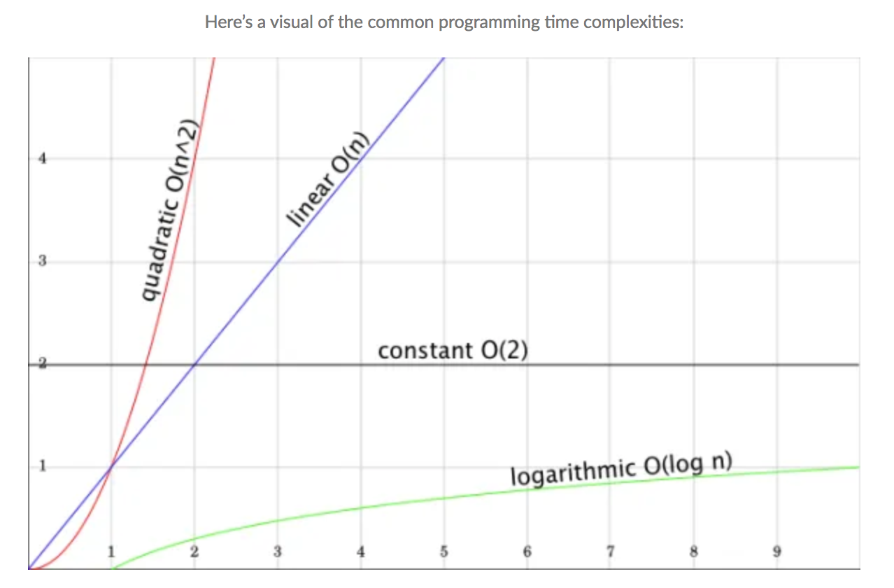
So, we have seen that the time complexity of current implementation is O(n^2) and know that O(n^2) bad (see graph below). Can we improve it?
Improving time complexity of current implementation of Dijkstra’s algorithm.
We will focus on the part of the algorithm that is making it quadratic, which is the while loop and it’s children (nested loops). We can’t avoid the requirement of visiting every node (done by while loop). We also can not avoid visiting each neighbours of a node during the relaxation process. What we can really look at is,
- Can we optimize the way we pick the lowest_cost node. Can it be done at a lesser cost that O(n).
All we are doing in find_lowest_cost_node() is to iterate over the costs_table entries, which is of time complexity O(n), to find the lowest cost node. Imagine, you have a queue where the lowest cost node is always placed at the front of the queue. Then, we can pick the cheapest node just by picking the first (front) element in the queue. The good thing is, such a queue is already there, which we call as priority queue, or min-heap. Now, the O(n) operation becomes O(1).
One important thing to keep in mind is that, the Priority Key implementation used in Dijkstra’s algorithm will have to support a special operation named decreaseKey(), which is basically used to update the priority of an already existing element in the priority queue. You may watch this excellent video by George T Heineman taken from his O’RELLY Video course Working with Algorithms in Python.
The pseudocode for Dijkstra’s algorithm with Priority Queue will look like this :
def shortestPath(G, s)
  PQ = new PriorityQueue
  set dist[v] ∞ for all v(of)G
  set pred[v] -1 for all v(of)G
  dist[s]=0

  foreach v(of)G
    PQ.insert(v, dist[v])

  while(PQ is not empty) do
    u = getMin(PQ)
    foreach neighbour v of u do
      w = edge weight of (u, v)
      newLen = dist[u] + w
      if (newLen < dist[v]) then
        decreaseKey(PQ, v, newLen)
        dist[v] = newLen
        pred[v] = u
Java implementation of Dijkstra’s algorithm
I think we have gained enough acquaintance with the Dijkstra’s algorithm that we can attempt it in Java now.
We will start with the naive approach and then go on to implement it with PriorityQueue.
package graph;

import java.util.*;

public class DijkstrasAlgo {

    public static void main(String args[]) {
//        graph = {
//                "Start" : {"A":6, "B":2},
//                "A" : {"Finish":1},
//                "B" : {"A":3, "Finish":5},
//                "Finish" : {}
//        }

        // Initialize the Graph
        Graph g = new Graph();
        g.addEdge("Start", "A", 6);
        g.addEdge("Start", "B", 2);
        g.addEdge("A", "Finish", 1);
        g.addEdge("B", "A", 3);
        g.addEdge("B", "Finish", 5);
        g.addVertex("Finish");

        System.out.println("Graph :"+ g);

        // We are passing null for endNode so that the algo will find
        // shortest path to all nodes.
        ResultPair<Map<String, Integer>, Map<String, String>> results =
                findShortestPath(g, "Start", null);

        System.out.println("CostsTable :" + results.resultOne);
        System.out.println("ParentsTable :" + results.resultTwo);

        // Let's print shortest path from Start to Finish and it's cost.
        System.out.println("\nPrinting path from Start to Finish.");
        String currentNode = "Finish";
        Deque<String> stack = new LinkedList<>();
        while(currentNode != null) {
            stack.push(currentNode);
            currentNode = results.resultTwo.get(currentNode);
        }

        while(stack.size() != 0) {
            currentNode = stack.pop();
            System.out.print(currentNode + "->");
        }

        System.out.println("\nCost of the path :"+ results.resultOne.get("Finish"));
    }

    public static ResultPair<Map<String, Integer>, Map<String, String>>
        findShortestPath(Graph g, String startNode, String endNode) {
        Objects.requireNonNull(g);
        Objects.requireNonNull(startNode);

        Map<String, Integer> costsTable = new HashMap<>();
        Map<String, String> parentsTable = new HashMap<>();
        Set<String> processedNodes = new HashSet<>();

        initializeCostsTable(g, startNode, costsTable);

        String leastCostNode;
        while((leastCostNode = findLeastCostNode(costsTable, processedNodes))
                != null) {
            if (leastCostNode.equals(endNode)) {
                break;
            }

            relax(g, leastCostNode, costsTable, parentsTable);
            processedNodes.add(leastCostNode);
        }

        return new ResultPair<Map<String, Integer>, Map<String, String>>
                (costsTable, parentsTable);
    }

    private static void initializeCostsTable(Graph g, String startNode,
                                             Map<String, Integer> costsTable) {
        Set<String> allVertices = g.getAllVertices();
        for (String vertex : allVertices) {
            costsTable.put(vertex, Integer.MAX_VALUE);
        }

        costsTable.put(startNode, 0);
    }

    private static void relax(Graph g, String leastCostNode,
                              Map<String, Integer> costsTable,
                              Map<String, String> parentsTable) {
        Map<String, Integer> neighbours = g.getNeighbours(leastCostNode);
        int costToReachLeastCostNode = costsTable.get(leastCostNode);
        for (String neighbourNode : neighbours.keySet()) {
            int edgeWeight = neighbours.get(neighbourNode);
            int newCost =  costToReachLeastCostNode + edgeWeight;
            if (newCost < costsTable.get(neighbourNode)) {
                costsTable.put(neighbourNode, newCost);
                parentsTable.put(neighbourNode, leastCostNode);
            }
        }
    }

    private static String findLeastCostNode(Map<String, Integer> costsTable,
                                            Set<String> processedNodes) {
        Integer leastCost = Integer.MAX_VALUE;
        String leastCostNode = null;
        for (String key : costsTable.keySet()) {
            if (processedNodes.contains(key)) {
                continue;
            }

            int cost = costsTable.get(key);
            if (cost < leastCost) {
                leastCost = cost;
                leastCostNode = key;
            }
        }

        return leastCostNode;
    }

    static class Graph {

        private Map<String, Map<String, Integer>> vertices =
                new HashMap<String, Map<String, Integer>>();

        public void addVertex(String vertex) {
            vertices.put(vertex, new HashMap<String, Integer>());
        }

        public void addEdge(String u, String v, int weight) {
            Map<String, Integer> neighbours =
                    vertices.getOrDefault(u, new HashMap<String, Integer>());
            neighbours.put(v, Integer.valueOf(weight));

            vertices.put(u, neighbours);
        }

        public Set<String> getAllVertices() {
            return vertices.keySet();
        }

        public Map<String, Integer> getNeighbours(String vertex) {
            return vertices.getOrDefault(vertex, new HashMap<String, Integer>());
        }

        @Override
        public String toString() {
            return "Graph{" +
                    "vertices=" + vertices +
                    '}';
        }
    }


    static class ResultPair<T, U> {
        private T resultOne;
        private U resultTwo;

        public ResultPair(T t, U u) {
            resultOne = t;
            resultTwo = u;
        }

        public T getResultOne() {
            return resultOne;
        }

        public U getResultTwo() {
            return resultTwo;
        }
    }
}
References
-
One of the best introductions on Dijkstra’s algorithm that I have come across is by Mr. Abdul Bari. It’s a YouTube video that’s available here.
-
George T Heineman’s George-T-Heineman video on Dijkstra’s algorithm is also very good to understand the implementation using priority queue.
-
An interesting stackoverflow discussion where I found this cool hipster4j library.
-
Finally, this is by far the best video that I have seen on Dijikstra’s algorithm. Probably I wouldn’t have seen anything else if I had gone through this one first.